4 Finding Genes with TSS-seq

The transcription start site (TSS) identifies the genomic position at which transcription begins. The first DNA-encoded nucleotide added to the RNA is designated +1. TSSseq is a technique specifically designed to identify the +1 genomic position for all transcription initiation events. To follow along with the text and to answer the “Test Your Understanding” questions, start with the “TSS-seq” session link. You can also use this link as a starting point to view TSS-seq data for any gene of interest.

4.1 What is TSS-seq?

RNAseq involves the sequencing of cDNA fragments derived from the mRNA present in a sample at the time of extraction. In this way, RNAseq attempts to identify all exons. TSS-seq is a special type of RNA sequencing that sequences cDNA fragments only derived from the 5′ ends of capped mRNAs present when RNA is extracted. Because all Pol II transcripts receive a 5′ cap during transcription, sequencing the cap-proximal region identifies the transcription start site (TSS). The steps necessary to prepare mRNA for TSS-seq are outlined in Figure 4.1. First, poly-A containing RNA (mRNA) is extracted as described previously (Figure 3.2). Due to the fragility of RNA, RNA extractions typically include full length mRNA (with a 5’ cap) and partially degraded mRNA (with a 5’ phosphate instead).

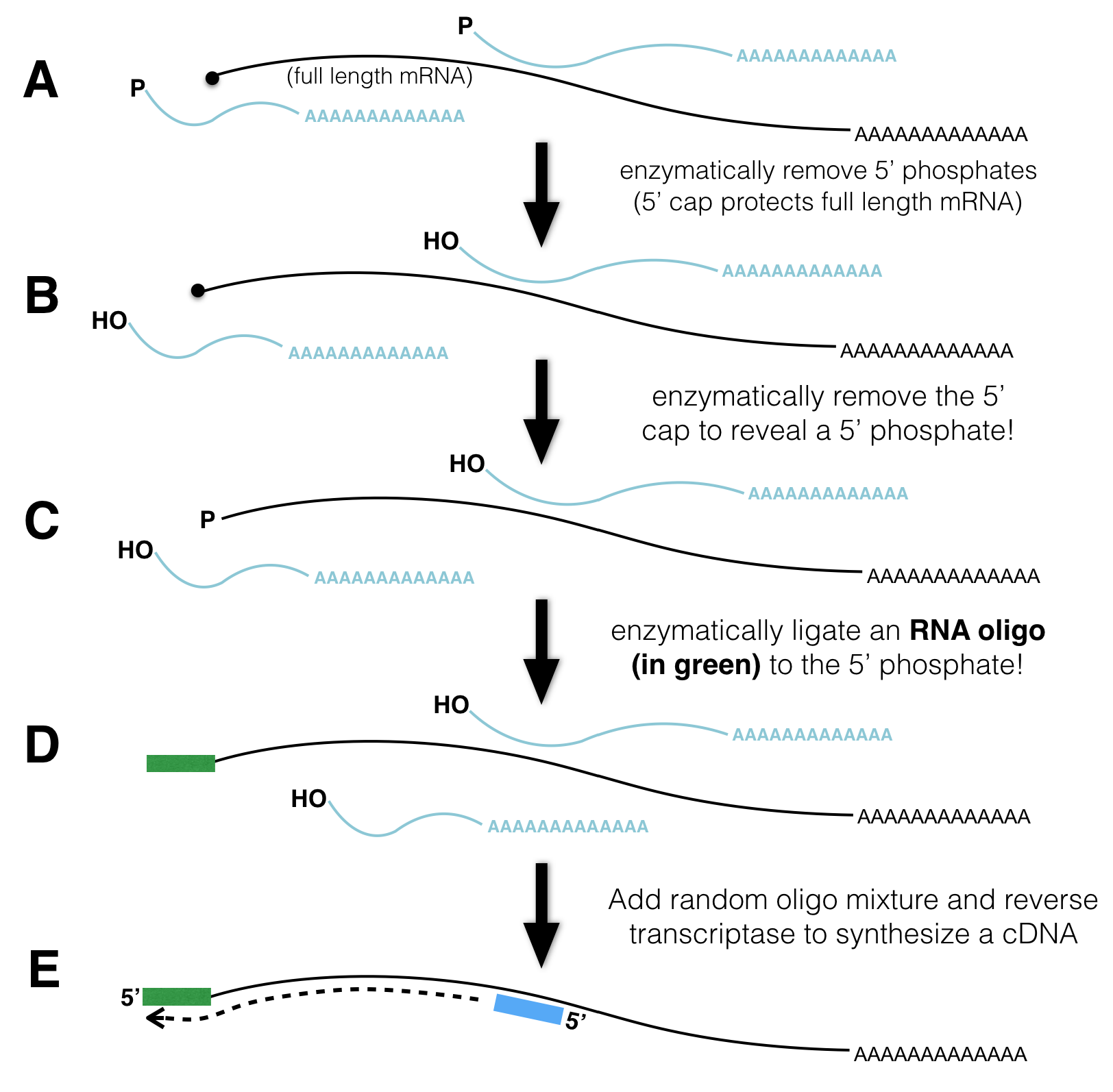
Figure 4.1: TSSseq protocol. A) All mRNA possessing a poly A tail is separted from total RNA. The resulting sample contains both full length mRNA with a 5’ cap and partially degraded mRNA with a 5’ phosphate (P-). B) An enzyme that removes 5’ phosphates is added. See the P change to OH. C) An enzyme is added that removes the 5’ cap structure. See the black circle change to a P. D) RNA ligase attaches an RNA oligo (green rectangle) to all RNAs that had a 5’ phosphate in C). E) The addition of reverse transcriptase and random oligos produce cDNA fragments. Those cDNA fragments that once had a 5’ cap all have the same sequence at their 3’ ends.

To distinguish full length mRNA from partially degraded fragments, an enzyme that removes 5’ phosphates from all partially degraded RNA molecules is added to the mRNA sample. Full-length, capped mRNAs do not possess a 5’ phosphate and are thus not affected by this enzyme. Now all the partially degraded mRNAs possess a 5’ hydroxyl. Next, an enzyme that removes the 5’ cap from full length mRNAs is added. Now, full length mRNAs that were once capped possess a 5’ phosphate (partially degraded mRNAs do not). Then, an RNA oligo²⁸ and RNA ligase²⁹ are mixed together. As a result, the single-stranded RNA oligo becomes ligated to the 5’ end of only those RNAs that have 5’ phosphates. Finally, reverse transcriptase and random primers are added. As a result, all the RNA in the tube is used as template to synthesize cDNA (complementary DNA). Importantly, only those cDNAs that once had a 5’ cap are tagged with a known sequence at their 3’ ends. This sequence tag can now be exploited for sequencing as the sequencing reaction is primed with a DNA oligo that hybridizes to the sequence tag. The short sequence reads that are collected are then computationally aligned to the genome.

4.2 How is TSS-seq useful?

As we saw in the previous chapter, RNA-Seq data can identify the position of exons, segments of the genome that were transcribed and remain in mRNA following splicing. RNA-seq data can also reveal how exons are linked together (with split alignments). That said, it is not always sufficient for gene identification purposes. To identify an individual transcription unit (a single gene) with more confidence, it is better to know the position of the exons and the TSS. To see this for yourself, review the RNAseq data corresponding to a small region of the genome (Figure 4.2). The NCBI Refseq gene prediction track is hidden on purpose. Can you determine how many genes are in this region? Why or why not?

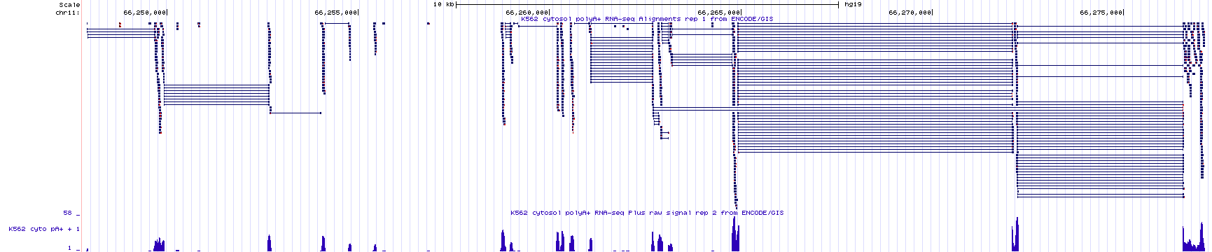
Figure 4.2: RNAseq data corresponding to a small region in the genome with the base position and gene prediction tracks hidden. Guess how many genes you think map to this region of the human genome. Continue reading below to discover the answer.

To see the true number of genes click here. This link takes you to the same genome region as in Figure 4.2 but with the gene prediction and base position tracks visible. Did you guess right?

4.3 How is TSS-seq Data Visualized?

The UCSC Genome Browser contains numerous evidence tracks displaying TSS-seq data. We will focus on one that was generated by the FANTOM5 Consortium of labs in Japan (FANTOM stands for Functional Annotation of the Mammalian Genome). Click the link to learn more about FANTOM5. To view this evidence track click the TSS-seq session link.

Your genome browser should now display the “Max Counts of CAGE³⁰ reads” evidence track for BBS1. This evidence track displays TSS-seq data in histogram form only (Figure 4.3). The track settings are configured so that the Y-axis maximum is set to an absolute value of 350 read counts. Setting the Y-axis maximum to 350 is sufficient for most genes. For highly expressed genes it is better to set the Y-axis to “auto-scale to data view”. Specifically, go to the track settings page. Scan down until you see “Data view scaling:”. Change the pulldown menu from “use vertical viewing range setting” to “auto-scale to data view”. Then click submit. If you do this for BBS1, the Y-axis should be considerably less. Before you move on, change the Y-axis back to “use vertical viewing range setting”. If you forget, you may notice that TSSseq data is noisy. Single sequence reads that map to random positions in the genome are plentifal and can be ignored.

Figure 4.3: TSSseq data for BBS1.

Zoom out 10X. The genome browser window is now focused on a larger portion of the genome surrounding BBS1 (Figure 4.4). Notice that there are both red peaks and blue peaks. There are also tall peaks and tiny peaks.

Recall that either DNA strand can serve as the template for transcription. If RNA polymerase uses the bottom strand as template then it moves from left to right (5’ to 3’) and produces an mRNA that matches the plus strand sequence and is complementary to the minus strand (the plus strand is the informational strand). If RNA polymerase uses the plus strand as template then it moves from right to left (also 5’ to 3’ relative to the minus strand) and produces an mRNA that matches the minus strand sequence (the minus strand is the informational strand). Histrogram peaks displayed in red represent TSSes for plus strand genes. Histogram peaks displayed in blue represent TSSes for minus strand genes.

The taller a histrogram peak at a given location, the more sequence reads that start at that spot. The more read counts, the more reliable the data and the more likely the data represents a true TSS. In fact, the tiny peaks observed in Figure 4.4 (find each red asterix) may reflect background noise³¹ and may not represent a true TSS. Moreover, the absence of a peak at a location where one is predicted to exist does not mean that the gene prediction is incorrect. This might be an instance where the gene was not expressed in the tissue sample that was used to generate the TSS-seq data. There is a common saying, “Absence of evidence is not evidence of absence”.

Figure 4.4: TSSseq data of a larger region surrounding BBS1. Each asterix (my annotation) highlights sequence reads that are not likely to represent true transcriptional start sites.

Now zoom in to the TSS for BBS1 (Figure 4.5). You can see that the position in the genome where the majority of experimentally defined TSSs are located is at the predicted transcriptional start site. This is not always the case. Also, notice that the transcriptional start sites for BBS1 are spread out to some degree. This is normal.

Figure 4.5: A close up view of the TSS-seq histogram data surrounding the predicted transcriptional start site for BBS1 (as defined by the NCBI refseq evidence track). The translational start site of BBS1 is shown in green.

Again, this is a great example of an evidence track that provides unbiased experimental evidence for the existence of a gene. It provides the position of all transcriptional start sites (TSS) within the genome. Each TSS identified by TSS-seq was not predicted to exist but was experimentally determined without prior knowledge (no bias).

That said, TSSseq data is not always sufficient to determine the number of individual genes in a given region of the genome. For example, review the TSS-seq histogram data in (Figure 4.6) and try to predict the number of genes in this region. I have omitted the gene prediction track to illustrate a point.

Figure 4.6: This is an image of the TSSseq evidence track for a small region of the human genome. All other tracks have been hidden. Count the number of transcription starts sites then guess how many genes you think these TSS peaks correspond to.

Now click here to see how many genes there really are in the genomic region shown in Figure 4.6. How does this differ from what you thought? Notice that the link has been configured to include the gene prediction track along with the RNA-seq and TSS-seq data tracks. Do you see how the RNA-seq data combined with the TSS-seq data provides a more complete picture of the true number of genes present? After all, there are genes that utilize alternative transcription initiation sites (Review (Chapter 2), “One gene, many splice variants”)!

4.3.1 Test Your Understanding

Some of the TYU questions will require the TSS-seq data displayed in the figure below (NOTE that the gene prediction track is hidden). To enlarge click on the image.

Click on the link above to see the questions.

4.4 Transcription Start Sites and the Core Promoter

One can assume that a transcriptional start site (TSS) identified by TSSseq, should reveal the site of a core promoter where general transcription factors (GTFs) bind and recruit RNA polymerase II. One well-studied core promoter motif is the *TATA-box, an A/T rich motif bound by the “TATA Binding Protein” (or TBP). TBP is a single polypeptide that is part of a larger protein complex, or GTF called TFIID. TBP/TFIID is required for all pol II transcription. TBP/TFIID binding initiates a cascade of events that ultimately leads to the formation of a preinitiation complex (PIC) at the TSS ((Figure 4.7).

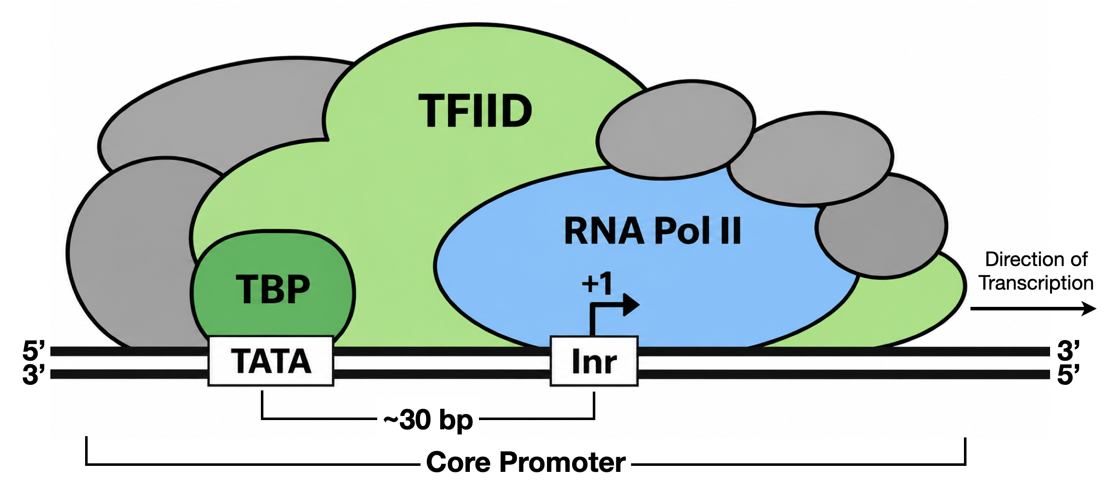
Figure 4.7: A simple schematic of a focused core promoter and the GTFs/RNA polymerase II that bind to it. The horizontal line is the genomic DNA. TATA, Inr, are the two most common DNA sequence motifs positioned found at the core promoter. Inr spans the TSS (+1) while the TATA-box is upstream of Inr.

Initially, the TATA-box was thought to be an essential core-promoter motif because it is the canonical binding site for TBP, a factor required for RNA polymerase II transcription initiation. We now know, however, that a TBP requirement does not imply a TATA-box requirement. In fact, a recognizable TATA-box is present in only a minority of human promoters, approximately 24%. The core-promoter motif found most often is the Initiator (Inr), which spans the TSS and contributes to TFIID recruitment. Surprisingly, nearly half of human promoters lack both a TATA-box and an Inr, indicating that TBP can be recruited through other promoter elements or combinations of elements that have yet to be described.

One reason our understanding of core-promoter sequence motifs remains incomplete is that it has been based largely on a limited set of experimentally tractable promoters, especially viral promoters and highly expressed cellular genes such as HBB. Many of these promoters exhibit focused transcription initiation, in which transcription begins predominantly at one or a few closely spaced TSSs. Consequently, the canonical motifs identified from these studies may not represent all RNA polymerase II promoters. In fact, a substantial fraction of mammalian promoters exhibit dispersed initiation, with transcription beginning across a broader region and often lacking a clearly defined combination of canonical core-promoter motifs. (Figure 4.8).

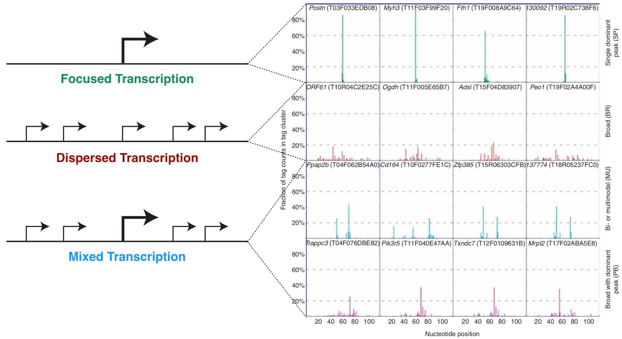
Figure 4.8: The left schematic from Vo ngoc et al. 2017 illustrates the three main types of promoters that are found in animals: Focused, Dispersed and Mixed. The right image from Carninci et al. 2006 displays TSS seq data for a number of genes that illustrate each type of promoter.

4.5 Consensus Sequences

The TATA-box and Inr were initially recognized as recurring sequence patterns in alignments of experimentally characterized core promoters, a strategy based on the principle that sequence conservation can reveal motifs important for factor binding. That said, sequence conservation is rarely absolute. By creating a multiple sequence alignment of a specific motif, one can evaluate the degree of conservation and create a consensus sequence. A consensus sequence (also known as a canonical sequence) can be defined as the “the most frequent residues, either nucleotide or amino acid, that are found at each position in a multiple sequence alignment” (Wikipedia). For a simple example, see Figure 4.9. Notice that the multiple sequence alignment contains only G, A, T and C while this consensus sequence contains additional letters (Y, N and R). Y,N and R belong to an agreed upon list of IUPAC nucleotide codes also known as IUPAC ambiguity codes. Here, Y = C or T, N = any nucleotide and R = G or A.

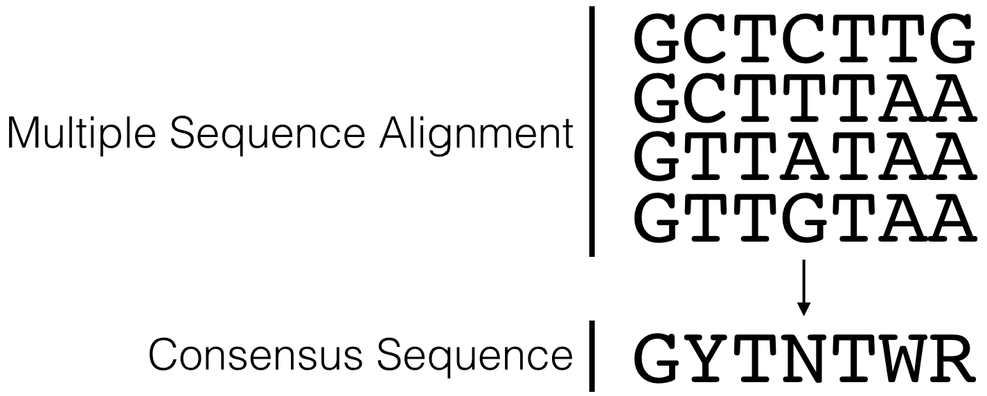
Figure 4.9: This is a simple multiple sequence alignment (MSA) that includes only 4 sequences. The consensus sequence corresponding to this alignment is written directly below. It was created by examining the observed frequency of each nucleotide present in each column of sequence in the MSA.

Figure 4.10 lists the consensus sequences for the TATA-box and the Inr.

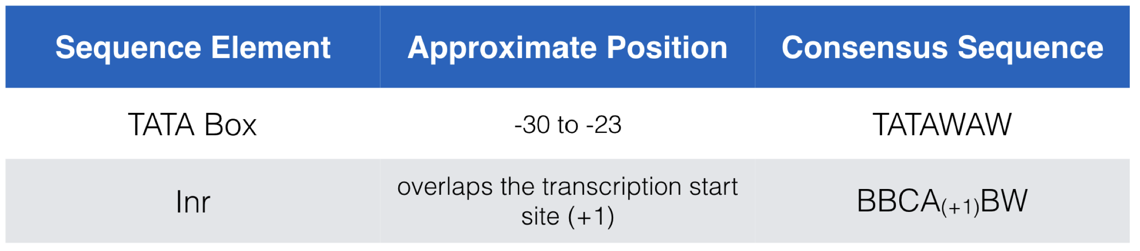
Figure 4.10: A list of the consensus sequences for the TATA-box and the Inr in mammals. Nucleotide positions listed in column 2 are all relative to the +1 position of the TSS. IUPAC codes in use include B=C/G/T and W=A/T.

In the UCSC genome browser, you can search for a consensus sequence containing IUPAC codes using an evidence track called, “Short Match”. Before you open Short Match, open the saved “TSS-Seq” Session then zoom in to view the sequence surrounding the TSS for BBS1. Now scroll down to find an evidence track entitled, “Short Match” (1) within the section entitled, “Mapping and Sequencing” (Figure 4.11). Change this evidence track from “hide” to “pack” and click “refresh” (2). A new evidence track will open (3). Click on the gray rectangle at left to open the track settings page for this track (4).

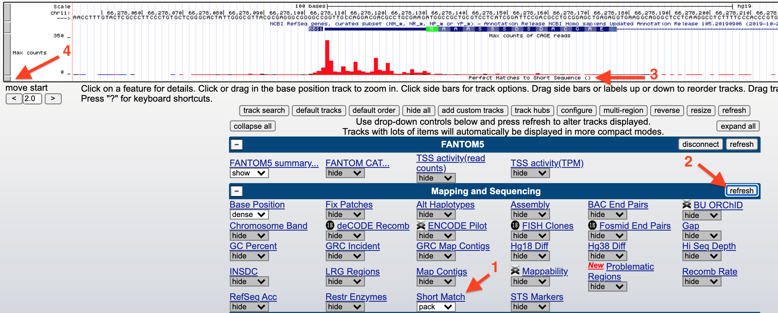
Figure 4.11: How to search for a consensus sequence: 1) change the Short Match evidence track from hide to pack. 2) Click Refresh. 3) A new evidence track will open. 4) Click on the gray rectangle to open the track settings page. Now see figure below.

Finally, input any sequence (i.e. ATG) into the search window (1) provided at the Track Settings page for Short Match (Figure 4.12) then hit “Submit” (2).

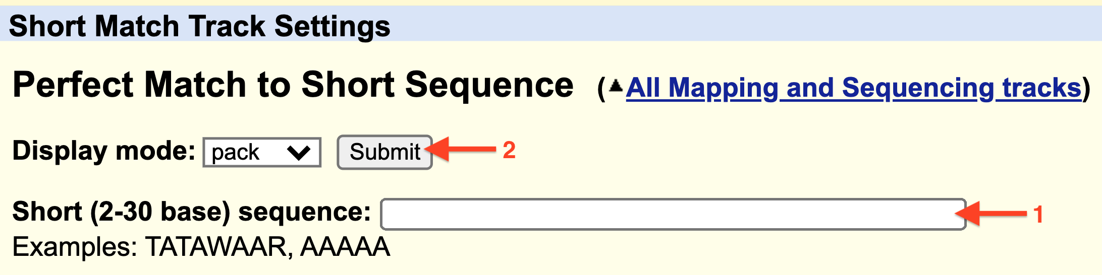
Figure 4.12: 1) Enter a consensus sequence in the window provided. 2) Click Submit.

In Figure 4.13, I searched for the Inr consensus sequence, BBCA(+1)BW, in the genomic region surrounding the human gene (CCT2) TSS. Each match is displayed in the Short Match evidence track as a thick black line. The position (i.e. 69,979,214) and orientation (- or +) of each match is written on the left of each line. In this example, the putative³² Inr is the one highlighted with a red asterisk. What is my evidence? This is the only Inr consensus sequence that spans the predicted and experimentally-defined TSS at position 69,979,236. It is also found on the plus strand of the genomic DNA and CCT2 is a plus strand gene. Finally, the “A” of the consensus sequence is positioned at the predicted and experimentally defined TSS (See red circle in Figure 4.13).

Figure 4.13: Horizonatal black bars within the ‘Short Match’ evidence track describe the position of each consensus sequence (BBCA(+1)BW) found within this genomic region. Information about the precise nucleotide position and orientation is provided on the left (see boxed consensus on the left). The putative Inr for CCT2 is highlighted with a red asterix. This consensus sequence is found on the plus strand (same as CCT2) and is positioned directly below the experimentally defined TSS at 69,979,236 with the A at the putative +1 position.

4.5.1 Test your understanding

Click the link above to see the TYU questions.

4.6 Sequence Logos

Sequence conservation, trends and patterns revealed by a multiple sequence alignment (MSA) can also be visualized with a “sequence logo” where the predominant residue is drawn as the tallest and placed at the top among all the residues found at a given position in an alignment. For example, let’s say at position 3 of an MSA there is a T in every single sequence (For a simple example see Figure 4.14). In a sequence logo, this would be displayed as a T of maximum height (illustrating that the T in that position is invariant and important). Now let’s say position 6 has an A in 75% of the sequences and a T in the remaining 25%. At this position of a sequence logo you would see an A on top of the T, the A would be proportionally larger than the T but the overall height of the two letters combined would be shorter than the T in position 3. And in the extreme case where G, A, T or C are found in equal proportion that position in the sequence logo would be left blank (see position 4 in Figure 4.14)! This indicates that that position of the alignment is utterly uninformative. In a traditional consensus sequence using IUPAC codes, this would be written as “N” for any nucleotide. One can also draw a sequence logo using frequency for the Y-axis. This type of sequence logo is more intuitive but many think it is less able to emphasize important sequence trends. What do you think?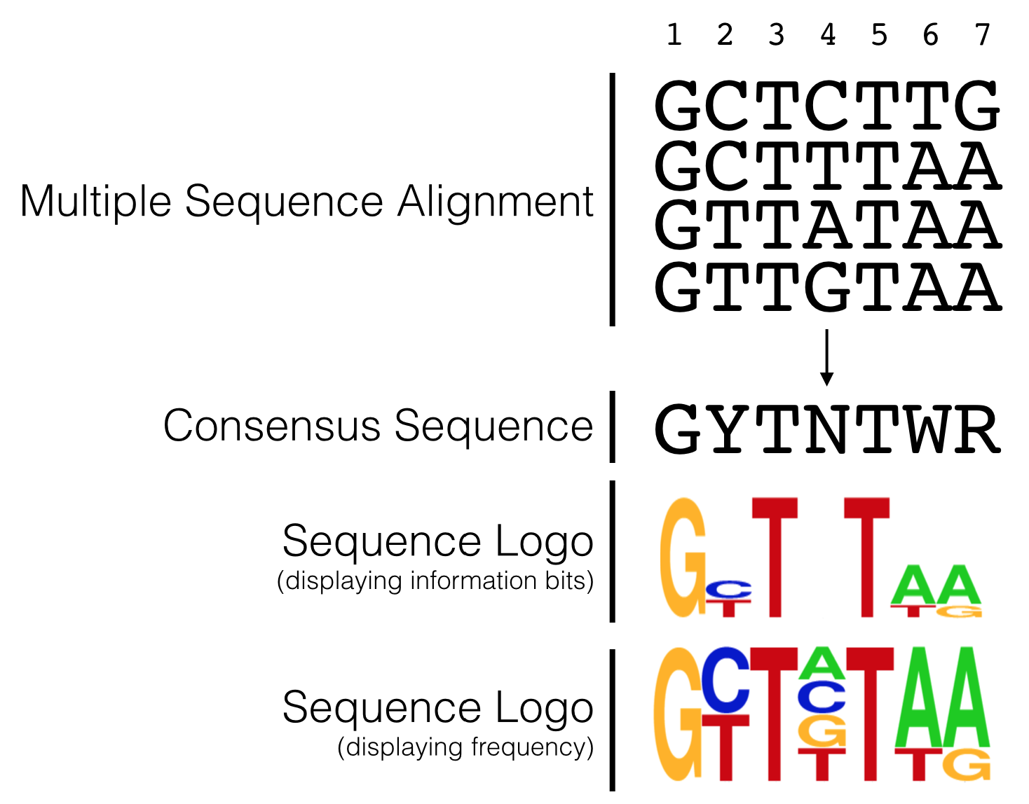

Figure 4.14: The hypothetical multiple sequence alignment is redrawn as a consensus sequence including IUPAC codes, or as a sequence logo with either information bits or frequency as the Y axis.

In 2006, Carninci et al. performed an unbiased, systematic analysis of all core promoter sequences identified by TSS-seq data obtained from RNA extracted multiple human tissue types. In their analysis confirmed the diversity of promoter types classifying them into four discrete categories (Figure 4.8) including the two extremes: Single Predominant Peak (SP) and Broad Peak (BR). They aligned core promoter sequences by category, placing the +1 position of the TSS in a single column then adding the surrounding sequences to create a large multiple sequence alignment. They then created a sequence logo for each multiple sequence alignment (MSA). Two are displayed in Figure 4.15. As you can see, the SP promoters are more likely to contain a TATA-box-like sequence about 30 nt upstream of the so-called Inr and there is a strong bias for a purine (G or A) at the +1 position of the TSS. Broad Peak (BR) promoters were found to be similar to SP promoters only in that they have a a strong bias for a purine at the +1 position of the TSS but they clearly lack a TATA-box and are enriched overall with Gs and Cs. Take home message: There are no universal promoter motifs. There may be sequence trends but there is a tremendous amount of sequence diversity at the core promoter. Clearly it would be very difficult to identify genes based solely on the presence of conserved core promoter sequence motifs.

What I have not discussed in this chapter is how a cell “knows” when and which tissue a gene should be transcribed. That requires far more than the core promoter sequence and can sometimes involves DNA sequence on other chromosomes! This is a topic for another course.

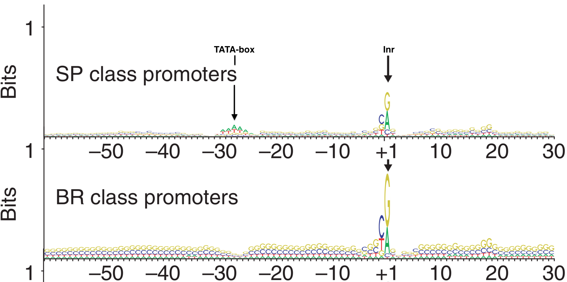
Figure 4.15: Sequence Logos for Single Predominent Peak (SP) and Broad Peak (BR) promoter types. The position of the TATA-box and Inr are highlighted in the SP class of promoters. The +1 represents the TSS.

4.6.1 Test Your Understanding

Click the link above to see the TYU questions.

4.7 Take Home Messages

• TSS-seq data is similar to RNA-seq data but with TSS-seq only the mRNA segment closest to the 5’ cap is sequenced.
  
• Whereas TSS-seq data identifies transcription start sites (TSS) of expressed genes, RNA-seq identifies exons.
  
• Finally, TSS-seq data combined with RNA-seq data is able to identify each transcription unit with more confidence.
  

© 2026, Maria Gallegos. All rights reserved.

---

28. Short single-stranded RNA chain↩︎

29. RNA ligase is similar to DNA ligase in that both require a 5’ phosphate and a 3’ hydroxyl to form a phosphodiester bond between two nucleic acid chains. The main difference: RNA ligase links two RNA chains together while DNA ligase links two DNA chains together↩︎

30. CAGE is short for ”Cap Analysis Gene Expression”↩︎

31. Molecular biology is messy. Each enzymatic step listed in Figure 4.1 is not likely to achieve 100% success. For example, partial mRNAs that fail to have their 5’ phosphates removed can be sequenced along side all the true full-length mRNAs.↩︎

32. potential, possible, not experimentally proven without a doubt but some evidence in support of the possibility↩︎